DC motors
Direct current (DC) motors are ubiquitous in control systems applications, from small hobby motors to industrial servo motors to electric vehicle traction motors. In this section, we will derive a mathematical model for a basic brushed DC motor from first principles, starting with the underlying electromagnetic laws. We will then make some idealizing assumptions to simplify the model for control design and analysis.
But first, let’s talk about the basics. A DC motor is a device that converts electrical power (voltage and current applied to input terminals) into mechanical power (torque and angular velocity of a spinning shaft). For this reason, we call DC motors electromechanical devices.


Figure 1:DC motor with input voltage , current , output torque , and angular velocity .
Electromagnetic principles
The key principle behind DC motors is how electric currents interact with magnetic fields to produce forces. This interaction is described by Lorentz’s force law[1], which states that a charged particle with charge moving with velocity in the presence of an electric field and magnetic field experiences a force (the Lorentz force) given by:
Let’s see how the Lorentz force leads to the operation of a DC motor. Consider what happens when we place a copper wire in a magnetic field and apply a voltage at either end of the wire to drive a current . The sequence of events is as follows:
The applied voltage causes an electric field to form that is aligned with the conductor, which causes a Lorentz force on the charged particles (electrons) in the wire. This force accelerates the electrons, causing them to flow; we get a current .
The moving particles now experience a Lorentz force due to the magnetic field. This force is perpendicular to both the direction of current flow and the magnetic field.
Since the charges are confined to the wire, the perpendicular Lorentz force is transferred to the wire itself, causing it to accelerate in a direction perpendicular to the current flow (Newton’s second law).


Figure 2:A wire carrying current in a magnetic field experiences a Lorentz force perpendicular to both the current and field. This causes the wire to accelerate upwards.
Slow electrons, fast current?
In metals, current is carried by electrons. In a vacuum, electrons can be accelerated to a substantial fraction of the speed of light. But in a wire, they move much more slowly due to collisions with atoms in the material. The average drift velocity of electrons in a typical copper wire is on the order of millimeters per second, even when the current is quite large! So why does current seem to flow instantaneously when we flip a switch? This is because the electric field that causes the electrons to move propagates along the circuit at a speed set by the geometry and surrounding materials, often a significant fraction of the speed of light. As this disturbance travels, electrons throughout the conductor begin to drift in response. Just like sound propagating through air, the individual air molecules move slowly, but the pressure wave moves quickly.
The wire is now accelerating, so the charged particles in the wire develop some upward velocity . This leads to an additional sequence of events:
By Lorentz’s force law, the charged particles now experience a Lorentz force , which points in the opposite direction to the current .
This force on the charges causes them to redistribute along the wire, creating a voltage that opposes the original voltage that caused the current . This induced voltage is also known as back EMF[2].
The back EMF reduces the net voltage across the wire, which reduces the current flowing through it, thereby reducing the force on the wire. Eventually, the wire reaches a steady velocity where everything is in balance.


Figure 3:A wire moving with velocity in a magnetic field experiences an induced voltage (back EMF) that opposes the applied voltage, reducing the current flowing through the wire.
DC motor construction
The basic principles described above can be exploited to produce rotational motion. The idea is to use a loop of current, which will produce torque that causes a shaft to spin. Here is a diagram showing the basic idea:


Figure 4:A current-carrying loop in a magnetic field experiences forces that produce torque, causing the loop to rotate.
From this basic principle, we can build a DC motor by arranging multiple current-carrying loops (windings) around a central shaft. Some useful terminology:
Stator: The stationary part of the motor that produces the magnetic field.
Rotor: The rotating part of the motor.
Commutator: A switching mechanism that changes the direction of current or the orientation of magnetic fields ensuring continuous torque in one direction.
All DC motors follow a similar causal chain of events:
The most common DC motor (small and cheap) is the permanent-magnet brushed DC motor (PMDC). It is most similar to the diagram of Figure 4:
the stator is a pair of permanent magnets that provide the constant magnetic field.
the rotor is a set of windings arranged around a central shaft.
the commutator is a mechanical switch that reverses the current direction every half-turn.
brushes (usually made of carbon) are pressed against the rotating commutator to transfer current from the external power source to the rotor windings and prevent the wires from getting tangled.
Here are two excellent videos that illustrate how a PMDC works. The first video gives a very basic introduction, while the second video goes into more detail about a particular design called a three-pole motor.
Video explaining how permanent-magnet brushed DC motors (PMDC) work.
Video going into more detail, specifically for three-pole PMDCs.
Types of DC motors
DC motors can be broadly classified into two categories based on how the commutation is achieved: brushed and brushless DC motors. The PMDC motor is an example of a brushed DC motor. Here are the defining characteristics of each type:
Brushed DC motors: These motors use mechanical commutation with brushes and a commutator to switch the current direction in the windings. They are simple, inexpensive, and easy to control, but require regular maintenance due to brush wear. Since large permanent magnets can be expensive, larger brushed DC motors often use wound-field stators, where the magnetic field is generated by electromagnets. Different types exist depending on whether the same power source is used for both the field and rotor windings (series, shunt, compound) or if they are powered separately.
Brushless DC motors: These motors do not use windings in the rotor, so brushes are not needed. Instead, the rotor has permanent magnets and the stator uses coils to produce a magnetic field. Sensors detect the rotor angle and a controller orchestrates rapid electronic switching of the stator magnetic field to produce torque (electronic commutation). Different topologies can be used for the rotor/stator depending on the application. Brushless motors are more efficient, have a longer lifespan, and require less maintenance than brushed motors, but are also more expensive.
DC motors in practice
Here are examples of different types of commercially available DC motors.
Permanent-magnet brushed DC motors (PMDC) are the most common type of small DC motor. They are inexpensive and simple to control, making them ideal for toys, small actuators, and automotive accessories. The example below is a small hobby motor. You can see the two permanent magnets on the stator. The rotor has seven poles, each with windings. You can also see the commutator with its seven segments and the brushes making contact on either side.
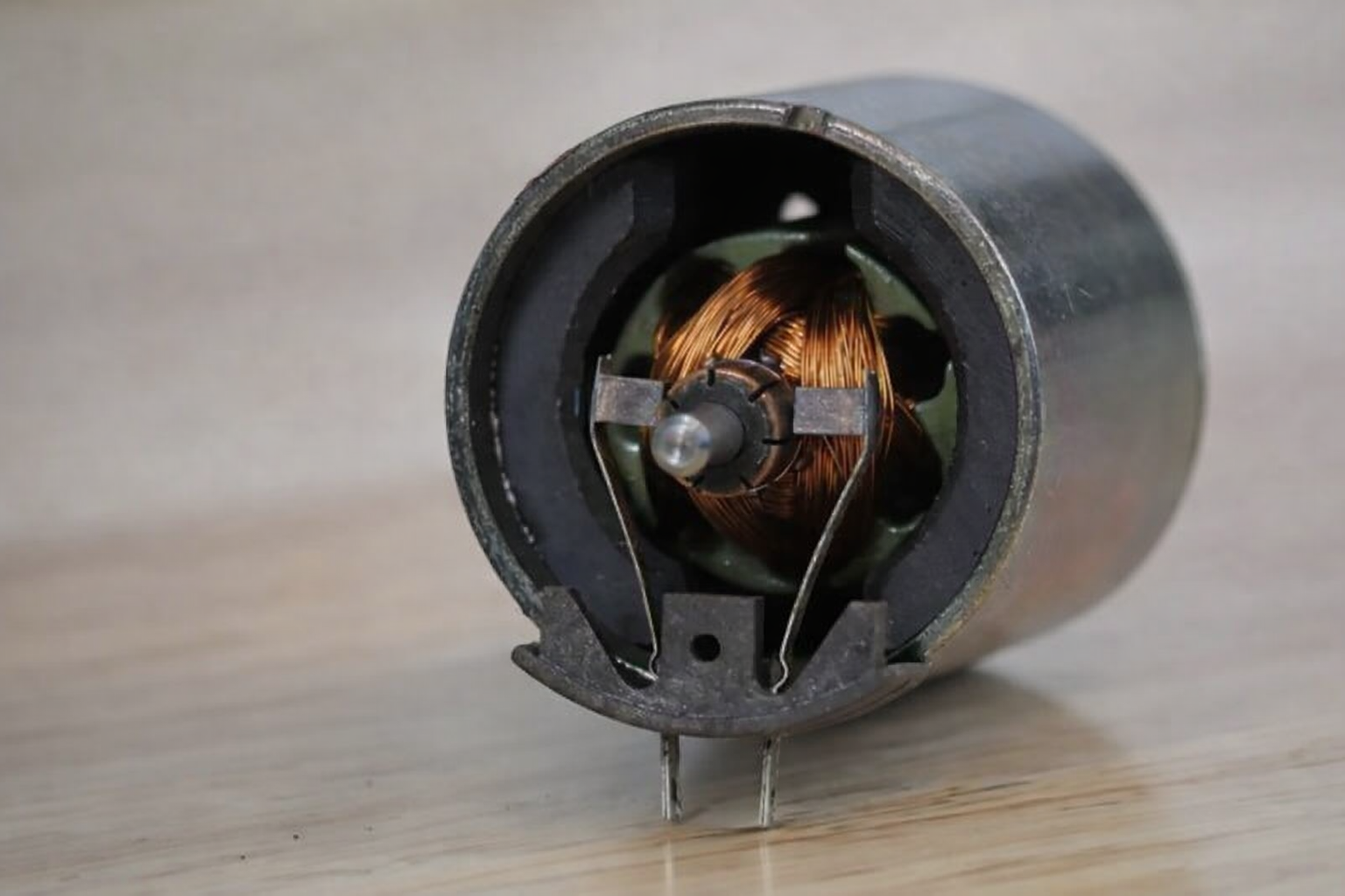
Permanent-magnet brushed DC motor (PMDC). Example: small hobby motor. Image credit: control.com.
The example below is also a brushed DC motor, but it has a wound-field stator instead of permanent magnets. This allows for a controllable magnetic field, which can be advantageous in larger industrial motors where permanent magnets would be too expensive. This example has many coils, as evidenced by the numerous segments on the commutator. Brushes are not shown.
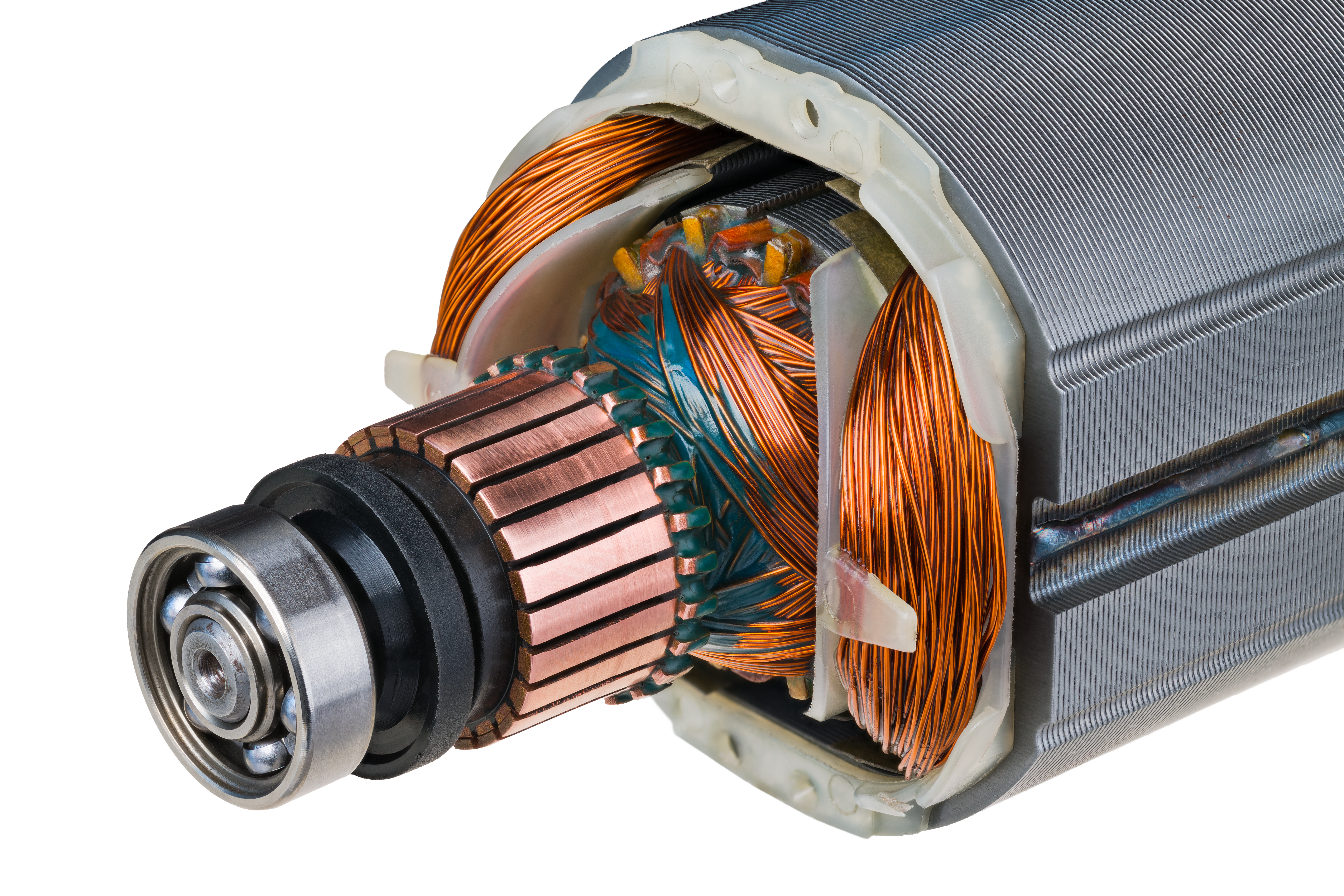
Wound-field brushed DC motor. Example: industrial motor with separately excited field. Image credit: Adobe Stock.
In brushless DC motors, the rotor typically contains permanent magnets, while the stator has the windings. The example below is a radial-flux brushless DC motor (BLDC) an inrunner topology, where the rotor is on the inside. This design is common in electric vehicle traction motors and power tools, as it can achieve high RPMs. You can see the permanent magnets lining the inside circumference of the rotor core.
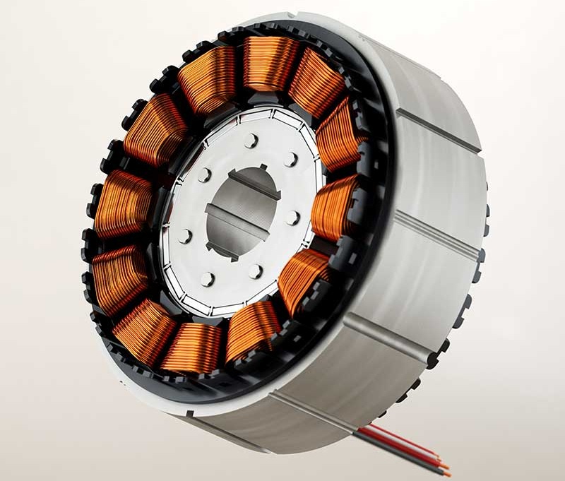
Permanent-magnet brushless DC motor (BLDC) with inrunner topology. Example: electric vehicle traction motor. Image credit: Magnetic Innovations.
Brushless DC motors can also have an outrunner topology, where the rotor is on the outside. This design provides high torque for its size, making it popular in applications like multirotor drones and gimbals. The example below also uses radial flux, but the permanent magnets are now on the outer shell of the motor. The entire black casing rotates while the coils inside remain stationary.
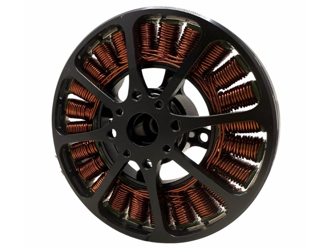
Permanent-magnet brushless DC motor (BLDC) with outrunner topology. Example: multirotor drone motor. Image credit: MechTex.
Another brushless DC motor topology is the pancake or axial-flux design, where the rotor is a disc that spins around a central axis. The coils have an axial rather than radial arrangement, and the permanent magnets are on arranged in a ring on the flat face of the rotor. This design can provide high torque in a slim profile, making it suitable for applications like electric vehicle performance motors and robot joints. The example below shows an example with a central rotor disc and stators with coils on either side.
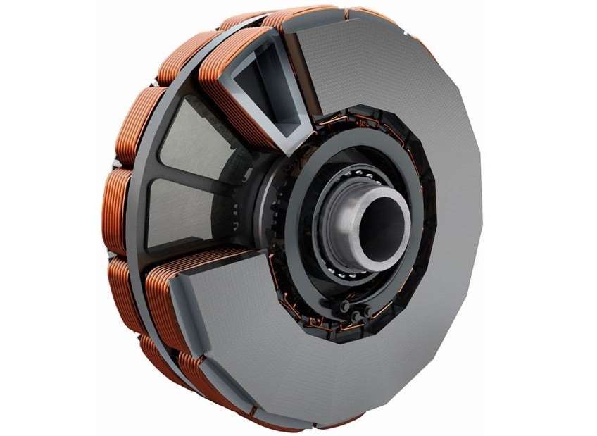
Axial-flux permanent-magnet brushless DC motor. Example: high-performance electric vehicle motor. Image credit: Whylot.
Here is a flowchart summarizing different types of DC motors with examples.
Figure 12:Flowchart of different types of DC motors.
Modeling a DC motor
We will develop a mathematical model for a basic permanent-magnet brushed DC motor (PMDC). The model consists of two main parts: the electrical dynamics governing the current flow in the motor windings, and the mechanical dynamics governing the rotation of the motor shaft. Here is a schematic diagram of the motor model we will use:


Figure 13:Model circuit for a brushed DC motor, showing electrical and mechanical components.
The windings are modeled as a series resistance and inductance , together with a back-EMF voltage source that opposes the applied input voltage . On the mechanical side, the motor produces a torque that must overcome a load torque through a rotor with inertia and viscous friction .
The inputs signals are the applied voltage and load torque .
The outputs signals are the motor angular velocity and current .
We will model the electrical and mechanical dynamics separately, and then combine them to obtain the complete equations of motion for the DC motor.
Electrical dynamics
The electrical dynamics are a straightforward RL circuit with two voltage sources: the applied voltage and the back-EMF voltage .


Figure 14:Model circuit for the electrical dynamics of a brushed DC motor. The windings have resistance and inductance , and there is a back-EMF voltage source opposing the applied voltage .
Examining Figure 14, applying the constitutive equations for the resistor and inductor yields the following differential equation:
The back-EMF voltage is proportional to the angular velocity of the motor shaft, so it satisfies a relationship of the form
where is the back-EMF constant of the motor, measured in volts per radian per second (V/(rad/s)), or volts per rpm (V/rpm). This constant depends on the motor construction, including the number of windings, magnetic field strength, and geometry.[3]
Mechanical dynamics
The mechanical dynamics are a rotational inertia (the rotor) with viscous friction and two torques: the load torque and the motor-produced torque .


Figure 15:Model for the mechanical dynamics of a brushed DC motor. The rotor has inertia and viscous friction , and experiences torques and .
Applying Newton’s second law for rotational motion to Figure 15 yields the following differential equation:
The motor-produced torque is proportional to the current flowing through the windings, so it satisfies a relationship of the form
where is the torque constant of the motor, measured in newton-meters per ampere (Nm/A). This constant also depends on the motor construction
Since the entire motor design can be boiled down to a single constant , we should talk a bit about what this constant means.
Equations of motion
The equations (2), (3), (4), (5), describe the dynamics of the DC motor. Let’s rewrite them here for convenience, and we’ll set to simplify the notation:
We can eliminate the variables and by substituting the second and fourth equations into the first and third equations, respectively. This yields the pair of ODEs:
In the next section, we will make some idealizing assumptions and solve modeling problems involving motors and other electromechanical devices.
Test your knowledge
Solution to Exercise 1 #
The two constants are the same, but they are expressed in different units. The speed constant is in rpm/V, To convert this to radians per second per volt, we can use the conversion factor :
The torque constant is given in Nm/A, which is the same as V/(rad/s). So based on this, the two constants should be reciprocals of one another. Let’s check:
This principle is distinct from Maxwell’s equations. Maxwell’s equations govern how electric and magnetic fields are generated by charges and currents and how the fields influence each other, while the Lorentz force law specifies how those fields exert forces on charged particles.
EMF stands for “electromotive force,” which is a historical term for voltage. Despite the name, EMF is not actually a force; it is measured in volts (V), not newtons (N).
Sometimes the relationship is written the other way, as , where is called the velocity constant, measured in (rad/s)/V or rpm/V.
- Hansen, P. (2022). On Automotive Electronics. ATZelectronics Worldwide, 17(9), 24–27. 10.1007/s38314-022-0821-1