Introduction

Engineers build machines that must behave reliably in the real world: temperatures drift, loads change, sensors are noisy, and everything has delay. Control is the set of ideas that lets us get predictable performance anyway: fast when we want fast, smooth when we want smooth, and stable when conditions change.

You already use control in everyday life: you choose a goal, take an action, observe what happened, and adjust. In this course we’ll take that familiar loop and turn it into engineering tools: simple diagrams to organize cause-and-effect, models that capture dynamics, and design methods that let you shape the response on purpose rather than by trial and error.

To make these ideas concrete, we’ll begin with a control problem you’ve solved hundreds of times, usually without realizing it.

Example: Shower temperature control¶

Imagine the simple task of adjusting a shower to a desired temperature $T_\textsf{des}$. We can adjust the knob angle $\theta$, which causes the temperature of the water $T_\textsf{true}$ to change. However, the change is not instantaneous, and we may imagine adjusting the knob over time, so we will write these quantities as functions of time: $\theta(t)$, $T_\textsf{des}(t)$, and $T_\textsf{true}(t)$.

It is useful to represent the temperature adjustment process as a block diagram (Figure 1).

The arrows in the block diagram indicate causality.

• $T_\textsf{des}(t)$ influences how I choose $\theta(t)$.

• $\theta(t)$ determines the future temperature of the shower $T_\textsf{true}(t)$.

Open-loop control¶

Since $\theta(t)$, $T_\textsf{des}(t)$, and $T_\textsf{true}(t)$ are functions of time, let’s make a plot of what these functions might look like. Here is one possibility:

At $t=0$, we decide to take a shower, and our desired temperature is $100\degree\textsf{F}$. We know from experience that $\theta(t) = 64\degree$ is the correct knob setting, so we turn the knob to that value and wait. But what if we wanted to reach $T_\textsf{des}$ more rapidly? Would that be possible?

Yes! To see why, let’s think about why the temperature responds the way it does. The hot water is stored in a tank, but the pipes that connect the tank to the showerhead are initially filled with cold water. The knob angle determines what mixture of hot water from the tank and cold water from the main supply line should be used. As time passes, the water in the pipes is replaced by the warm mixture from the tank and the main line. This warm water gradually heats the pipes, which eventually reach the same temperature as the warm water. At this point, the pipes cease to cool the water and the showerhead temperature reaches an equilibrium. We might expect these changes to occur at a rate proportional to the temperature difference (Newton’s law of cooling).

Of course, this is an approximate model, which we could verify more rigorously with experiments, but let’s go with it for now. We should expect that more hot water should lead to proportionately faster heating, so something like this:

This suggests that we could reach our goal faster if we used a clever switching strategy. First, we should use as much hot water as possible, and then we should back off before the water gets too hot. Something like this:

This switching strategy does heat the water faster, but we waited too long before turning the knob, which led to overshoot. Some tuning would be required to make this perfect.

This sort of control approach is called open-loop control: we decide on our course of action $\theta(t)$ in advance, and then we apply it. It doesn’t require much effort (just following a recipe), but it is generally fragile:

• The switching time must be calibrated, and might change from day to day. For example, the pipes might already be warm because somebody else took a shower recently.

• We chose $64\degree$ as the final knob angle “from experience,” but what if a visitor is using your shower and prefers the water to be at $95\degree\textsf{F}$ rather than $100\degree\textsf{F}$? How would you know what knob angle to recommend?

• Even if you know the knob angle on a given day, what if this value changes depending on the time of year? During the winter, the cold water from the supply line might be extra cold. What if someone flushes a toilet or another shower turns on while you’re taking your shower?

• Finally, our strategy wouldn’t work on a different shower in a different building. We would need to re-calibrate every time.

In other words, open-loop control works only to the extent that your model (and calibration) matches reality.

In practice, nobody does this... because we use feedback!

Closed-loop control¶

The more sensible approach is to place your hand in the water stream (measure the temperature). If the water is too cold, increase the knob angle. If the water is too hot, decrease the knob angle. This basic principle is called feedback, and it leads to a strategy called closed-loop control. Here is an updated diagram:

Some notes on how to read this block diagram:

• When two signals split apart (e.g., right after the shower), they are duplicated. So the signal entering the hand block is $T_\textsf{true}(t)$.

• When two signals come together, we use a junction. If the junction is unlabeled, it is assumed the signals are just added together. If you see small $+$ or $-$ signs next to the junction inputs, this indicates how the corresponding signals should be added together. For example, in Figure 5, the junction tells us that

  $$\Delta T(t) = T_\textsf{des}(t) - T_\textsf{meas}(t)$$

  (1)

• Ideally, we would have $T_\textsf{meas}(t) = T_\textsf{true}(t)$, but in reality, there might be error due to the fact that the hand is not always a reliable sensor.

The “me” block is now acting on the error, and there are two cases:

1. $\Delta T(t) > 0$. This occurs if $T_\textsf{des}(t) > T_\textsf{meas}(t)$, meaning the water is not hot enough, so we should increase the knob angle $\theta(t)$.

2. $\Delta T(t) < 0$. This occurs if $T_\textsf{des}(t) < T_\textsf{meas}(t)$, meaning the water is too hot, so we should decrease the knob angle $\theta(t)$.

Here are two popular ways to adjust knob angle based on the error signal:

• Bang-bang control: We either turn the knob all the way hot or all the way cold, and use a margin (also known as a deadband, or hysteresis). For example:

  $$\theta(t) = \begin{cases} \theta_\textsf{max} & \textsf{if } \Delta T(t) > 2\degree\textsf{F} \\ \theta_\textsf{min} & \textsf{if } \Delta T(t) < -2\degree\textsf{F} \\ \end{cases}$$

  (2)

  Bang-bang control is often used when the system can only be turned on or off, such as many residential heating units. This is how thermostats often work.

• Proportional control: We turn the knob an amount proportional to the error:

  $$\theta(t) = \theta_0 + k\, \Delta T(t)$$

  (3)

  Here, $k>0$ is called the proportional gain. Generally, $k$ is a constant that we pick ahead of time (this is called tuning). Using a larger $k$ usually yields a faster response, but picking $k$ too large can cause problems (we’ll learn more about this later!).

The benefit of using feedback control as in Figure 5 (instead of open-loop control as in Figure 1) is that it is far more robust. As we know from personal experience, this approach works for a variety of showers, regardless of personal temperature preference or external factors such as time of year.

Automatic control¶

It is often possible to automate a control process so that a human need not be involved. Typically, the “hand” is replaced by a sensor, and the “me” block is replaced by some sort of digital computer or software. A mechanical actuator would also be needed to adjust the knob so no human intervention is needed. Once this is done, the human only needs to choose the desired temperature and the rest happens automatically! Here is an updated diagram:

The power of a control system as in Figure 6 is that the user does not need to know anything about the inner workings of the shower, Newton’s law of cooling, knob calibration, or any complications due to external factors. The user simply picks their desired temperature and the control system handles everything automatically.

More examples¶

Why stop at showers? The idea of feedback can be used to control just about anything. Control systems can be used to improve the efficiency, safety, and performance of systems. In fact, many engineered systems in use today would be impossible to control if humans had to control them manually. Look no further than Wilbur Wright (one of the Wright brothers, who invented, built, and flew the first successful airplane.)

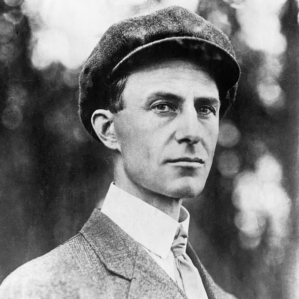
“As long ago as 1884 a machine weighing 8,000 pounds demonstrated its power both to lift itself from the ground and to maintain a speed of 30 to 40 miles per hour, but failed of success owing to the inability to balance and steer it properly. This inability to balance and steer still confronts students of the flying problem, although nearly eight years have passed. When this one feature has been worked out, the age of flying machines will have arrived, for all other difficulties are of minor importance.”

By the way, it was two years later, in 1903, that the Wright brothers would complete their historic first flight. Airplanes became a significant military capability by World War I (1914-1918), and became common for passenger travel in the 1930s.

Virtually anything can be viewed as a system. Applying feedback produces a control system. There are countless examples... Here is a partial list.

The above examples are related to mechanical engineering, which will be our primary focus. However, this class will teach you to view everything as a system. So the techniques you learn will be broadly applicable beyond mechanical engineering use cases.

Some of the control systems listed above are not engineered systems; they occur in nature. So understanding the fundamental principles of control systems can also help in understanding how systems in science and nature function.

Class overview¶

There are three chapters in this class.

1. Modeling

   • Use principles from physics (Newton’s law, Ohm’s law, Hooke’s law) to build a mathematical model (typically differential equations) that relates the inputs to the outputs. The first step in controlling a system is modeling it.

   • We will see how to do this for various mechanical, electrical, electromechanical, hydraulic, and thermal systems.

2. Analysis

   • Given a mathematical model of a system, predict and/or simulate how it will respond to a given input.

   • Develop intuition for different broad classes of systems.

   • Develop metrics to quantify the performance of a system.

3. Control

   • Learn how to change the dynamic response of a system by using feedback control, and which control strategies are appropriate for which types of systems.

   • Learn about trade-offs and fundamental limits of what is possible.

We will cover these topics both analytically and computationally. In other words, we will:

• Learn to use mathematical tools (algebra, calculus, complex analysis) to develop intuition for simpler control systems when possible, and

• Use computational tools (MATLAB) to solve more complex examples numerically.

Let’s get started!