Linear mechanical systems

Newton’s laws¶

In this lecture, we consider mechanical systems with translational motion in one direction. The most important facts we will use are Newton’s laws. The fundamental physical object in this context is a particle, which carries a constant mass $m$ and has (vector) position $\x(t)$.

Since we will be dealing extensively with functions of time (also called signals), we will use two notation conventions so that our equations do not look too cluttered.

• We use dots to denote time derivatives, so we write $\dot \x(t)$ instead of $\frac{\dd}{\dd t}\x(t)$ and we write $\ddot \x(t)$ instead of $\frac{\dd^2}{\dd t^2}\x(t)$. We can also write $\dot{\ddot{\x}}(t)$ and $\ddot{\ddot{\x}}(t)$ for higher derivatives.

• We often omit the $(t)$ for brevity. Therefore, it is important to know based on the context which symbols represent fixed parameters, such as the mass $m$, and which represent signals, such as the position $\x(t)$.

We will now specialize Newton’s laws to rigid body motion in 1D. A rigid body is a large collection of particles that are constrained to keep the same relative position to one another. In 1D, we assume the body only translates in one direction (no rotation), and all external forces are applied in that direction. In this case, all points on the body have the same velocity $\dot x$ and acceleration $\ddot x$, and the quantities $\dot x$, $\ddot x$, $F_i^\textsf{ext}$ may be treated as scalars since they only act in 1D. If the total mass of the body is $m$, Newton’s second law simplifies to:

In other words: In 1D, the mass of a body times its acceleration is equal to the sum of all external forces acting on the body. For a detailed derivation, see the appendix on Newton’s laws.

Fundamental components¶

Stiffness elements¶

A stiffness element is used to represent a spring-like interaction between two points. If you apply a force to compress or stretch the space between the two points, the stiffness element deforms accordingly, and acts as a lossless energy storage device. We represent stiffness elements as a zig-zag line, which depicts a spring.

In the diagram of Figure 1, we have:

• The arrows labeled $F$, which indicate that a force $F(t)$ is being applied in opposite directions on both ends of the spring. We omit the $(t)$ for brevity, but you should always assume that applied forces (or system inputs in general) could be functions of time.

• Measurements $x_1(t)$ and $x_2(t)$ with corresponding arrows that indicate direction. This tells us how we will record/track the positions of the endpoints of the spring. These are measured with respect to fixed inertial space. For example, the arrow to the right means that the left endpoint is displaced an amount $x_1$ to the right. So if $x_1>0$, the point moves right, and if $x_1<0$, the point moves left.

• Finally, the spring is labeled $k$ to indicate that this is the spring constant of the spring and that it obeys Hooke’s Law: the force is proportional to the displacement.

  $$F = k (x_2 - x_1)$$

  (2)

  This sort of equation relating different physical quantities is called a constitutive equation. The minus sign is there because $x_2-x_1$ represents the lengthening of the spring. The spring lengthens if $x_2>0$ (the right point moves right) or $x_1<0$ (the left point moves left). Note that if $x_1=x_2=5$, for example, both endpoints move right 5 units, so there is no net lengthening!

We can also have one endpoint fixed, which we represent using a line with hash marks.

In this case, the left endpoint of the spring is fixed to the wall, so we do no need to label it, and Hooke’s law simply becomes $F=kx$.

Damping elements¶

A damping element is used to represent a dashpot-like (viscous) interaction between two points. If you apply a force to compress or stretch the space between the two points, the damping element deforms at a speed that depends on the force, and acts as an energy dissipation device. We represent damping elements as a cartoon-like piston, which depicts a dashpot.

Another damping element is viscous friction, which happens when there is a viscous fluid at the interface between two surfaces that causes the two surfaces to slide at a speed that depends on the tangential force applied. We represent this as a hatched region between the surfaces. The two damping elements are depicted below.

Both of the damping elements shown in Figure 3 have the same constitutive equation:

Free body diagrams¶

To obtain equations of motion for an interconnected system involving masses, stiffness, and damping elements, we apply Newton’s second law once for each inertia (each mass) in the system. A simple way of keeping track of the various forces at play is to draw a free body diagram for each inertia.

When connecting elements together, we apply Newton’s third law. This means that our stiffness (or damping) elements can be interpreted in two different ways:

1. When you apply a force $F$ to a spring, it deforms an amount $x$, where $F=kx$.

2. When you deform a spring an amount $x$, it resists with a force $F$, where $F=kx$.

So when we connect a spring to a mass, the force that the mass imparts on the spring will be equal and opposite to the force the spring imparts on the mass.

Example: spring-mass-damper¶

Consider the classical spring-mass-damper system shown in Figure 4.

Car suspension

A common example of a spring-mass-damper system is a car suspension, which typically consists of an inner tube surrounded by a coiled spring, as shown below.

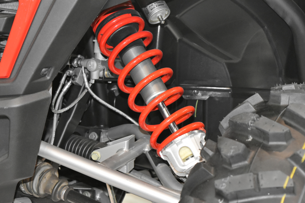
The outer coil is an ordinary spring. The inner tube is a damper, more precisely a hydraulic shock absorber: a piston in an oil-filled cylinder, where oil is forced through valves/orifices, dissipating energy and resisting relative motion.

There is a single inertia (the mass $m$) connected to a wall by a spring and a damper. The wheels under the mass indicate that there is no friction. There is also an external force $f$ applied to the mass.

The spring and damper exert forces on the mass, so let’s draw a free body diagram of mass $m$ to account for all the forces:

The spring force $f_s$ and damper force $f_d$ are drawn pointing in the direction we expect them to act when $x>0$. A displacement to the right ($x>0$) will cause the spring to exert a force on the mass towards the left (resisting the motion). As we will see later, it doesn’t matter which way you draw these arrows, as long as you adjust your constitutive equation accordingly!

We can now write all the relevant equations:

Eliminating $f_s$ and $f_d$ by substituting the two constitutive equations into Newton’s law and rearranging the equation, we obtain our final equation of motion:

Sign conventions¶

The directions of the arrows in the free body diagram are a convention. The arrow says “this is the direction we’ll be calling positive”. This does not mean the force must act in this direction! If it acts in the opposite direction, it will simply have a negative value.

What happens if we use a different convention in the spring-mass-damper system? Let’s draw our FBD differently this time, by switching the direction of the spring force.

The relevant equations now become:

The spring equation changes because when we have a positive displacement ($x>0$), the spring force should oppose the motion ($f_s<0$). Newton’s second law also changes because $f_s$ is now aligned with $x$. The two effects cancel out, and we obtain the same equation of motion as before, (5).

More examples¶

For the rest of this lecture, we will cover several different examples. Each uses a similar workflow to the spring-mass-damper system of Figure 4, but with increasing complexity.

Example: springs in parallel¶

Consider two springs connected in parallel to a mass.

The relevant equations for this system are:

Eliminating $f_{s1}$ and $f_{s2}$ by substitution, we obtain our equation of motion:

Example: springs in series¶

Now consider two springs connected in series to a mass.

The difficulty here is that if we draw a free body diagram for mass $m$ only, we will not have enough information to solve the problem. This is because the displacement of the seconds spring is $x-z$, so our equation of motion will depend on both $x$ and $z$.

The trick to solving this problem is to imagine a fictitious mass $m_0$ located between the two springs. Let’s now make free body diagrams for both masses:

The relevant equations for this system are now:

Eliminating $f_{s1}$ and $f_{s2}$ by substituting into last two equations, we obtain

Setting $m_0=0$ in the first equation, the differential equation becomes an algebraic equation (no derivatives). We can solve for $x$ and obtain:

Plugging this back into (10) and simplifying, we obtain our equation of motion:

Test your knowledge¶

Solution to Exercise 1 #

Begin by drawing the free body diagrams for both masses.

The force $f_d$ corresponds to the viscous friction force, which acts equal and opposite on the two masses. The spring forces $f_{s1}$ and $f_{s2}$ were drawn so as to oppose the directions of $x_1$ and $x_2$, but again, this is just a convention and has no effect on the final answer. Now, we can write our system of equations.

$$\begin{aligned} f_{s1} &= k_1 x_1 && \textsf{(first spring)}\\ f_{s2} &= k_2 x_2 && \textsf{(second spring)}\\ f_d &= b(\dot x_1-\dot x_2) && \textsf{(viscous damping)}\\ m_1 \ddot x_1 &= -F_a -f_{s1} -f_d&& \textsf{(first mass)}\\ m_2 \ddot x_2 &= -f_{s2}+f_d && \textsf{(second mass)}\\ \end{aligned}$$

(13)

The trickiest part is getting the signs right on the viscous damping. One way to do this is to imagine displacing one mass while holding everything else fixed.

• Look at $m_1$. Imagine holding $m_2$ fixed ($x_2=0$) and moving $m_1$ in the positive-$x_1$ direction. We would expect the friction force to oppose the motion, so $f_d = b \dot x_1$, since the $f_d$ acting on $m_1$ is already opposing the direction of $x_1$.

• Now look at $m_2$. Imagine holding $m_1$ fixed ($x_1=0$) and moving $m_2$ in the positive-$x_2$ direction. We would expect the friction force to oppose the motion, so $f_d = -b \dot x_2$, since the $f_d$ acting on $m_2$ is in the same direction as $x_2$.

When neither mass is held fixed, the system obeys superpostion; we can just add the two friction forces together and obtain $f_d = b(\dot x_1-\dot x_2)$.

Returning to Eq. (13), we can substitute the first three equations into the last two equations to eliminate $f_{s1}$, $f_{s2}$, and $f_d$, and we obtain:

$$\boxed{\begin{aligned} m_1 \ddot x_1 + b(\dot x_1 - \dot x_2) + k_1 x_1 &= -F_a \\ m_2 \ddot x_2 - b(\dot x_1 - \dot x_2) + k_2 x_2 &= 0 \end{aligned}}$$

(14)