RLC circuits
Electrical circuits that contain a power source (voltage or current source) together with resistors (R), inductors (L), and capacitors (C) are known as RLC circuits.
RLC circuits are fundamental in electrical engineering and physics, as they can model a wide range of dynamic behaviors, including oscillations and transient responses. The interplay between resistance, inductance, and capacitance gives rise to rich dynamics that can be analyzed using differential equations.
Components and constitutive equations
Circuits are made of components connected by wires. Electric charge () is measured in coulombs (C), and current (), the rate of flow of electric charge, is measured in amperes (A), which are coulombs per second. Current flows through a circuit much like water flows through pipes. In this analogy, water volume corresponds to electric charge, and water flow rate corresponds to electric current. The pipes are the wires and components of the circuit.
Current is caused by differences in electric potential, or voltage. Electric potential is analogous to pressure in a fluid system; just as water flows from high pressure to low pressure, electric charge flows from high potential to low potential. Voltage () is measured in volts (V).
Each component in an RLC circuit has a specific relationship between the voltage drop across it and the current flowing through it, known as its constitutive equation. The following figure shows the components of an RLC circuit and their constitutive equations.


Figure 1:Components of an RLC circuit and their constitutive equations.
RLC components in practice
RLC components come in many shapes and sizes, depending on their ratings and applications. Click the tabs below for more information on each component type.
Resistors are made from a variety of materials. The most common are carbon. They are designed to provide a specific resistance value and can handle varying amounts of power dissipation (power is the product of current and voltage drop). Resistors dissipate power as heat, so more dissipation usually requires physically larger resistors. Resistance is measured in ohms (Ω) and typically span a wide range from single-digit ohms to megaohms (MΩ).
The image below shows different types of resistors. Potentiometers and rheostats are variable resistors whose resistance can be manually adjusted. For the carbon resistors, the color bands indicate their resistance value and tolerance. See here for a guide on reading resistor color codes.
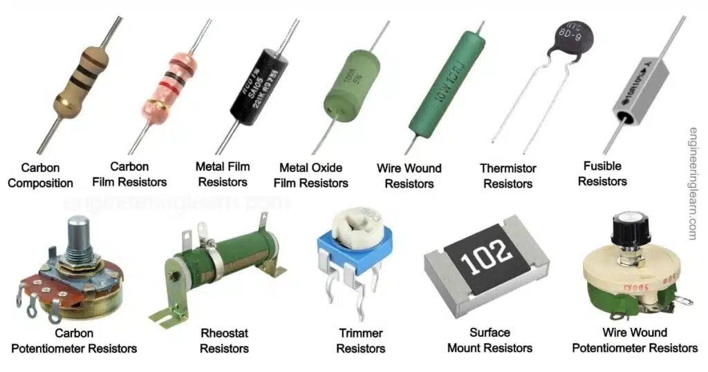
Different types of resistors. Image credit: engineeringlearn
Capacitors come in many shapes and sizes, depending on their capacitance value, voltage rating, and application. The most common are ceramic (small and flat) and electrolytic (look like miniature batteries). Capacitance is measured in farads (F), but practical capacitors are often in microfarads (μF), nanofarads (nF), or picofarads (pF) due to the large size of a farad. Larger capacitance values typically require physically larger capacitors. The image below shows different types of capacitors.
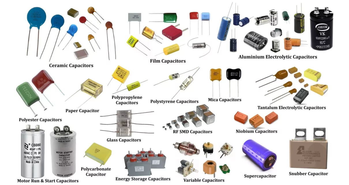
Different types of capacitors. Image credit: hackatronic.com
Inductors are typically made by winding a coil of wire around a core material, which can be air, iron, or ferrite. The core material affects the inductance value and the inductor’s ability to handle current without saturating. Inductance is measured in henrys (H), but practical inductors are often in millihenrys (mH) or microhenrys (μH) due to the large size of a henry. Larger inductance values usually require physically larger inductors. The image below shows different types of inductors.
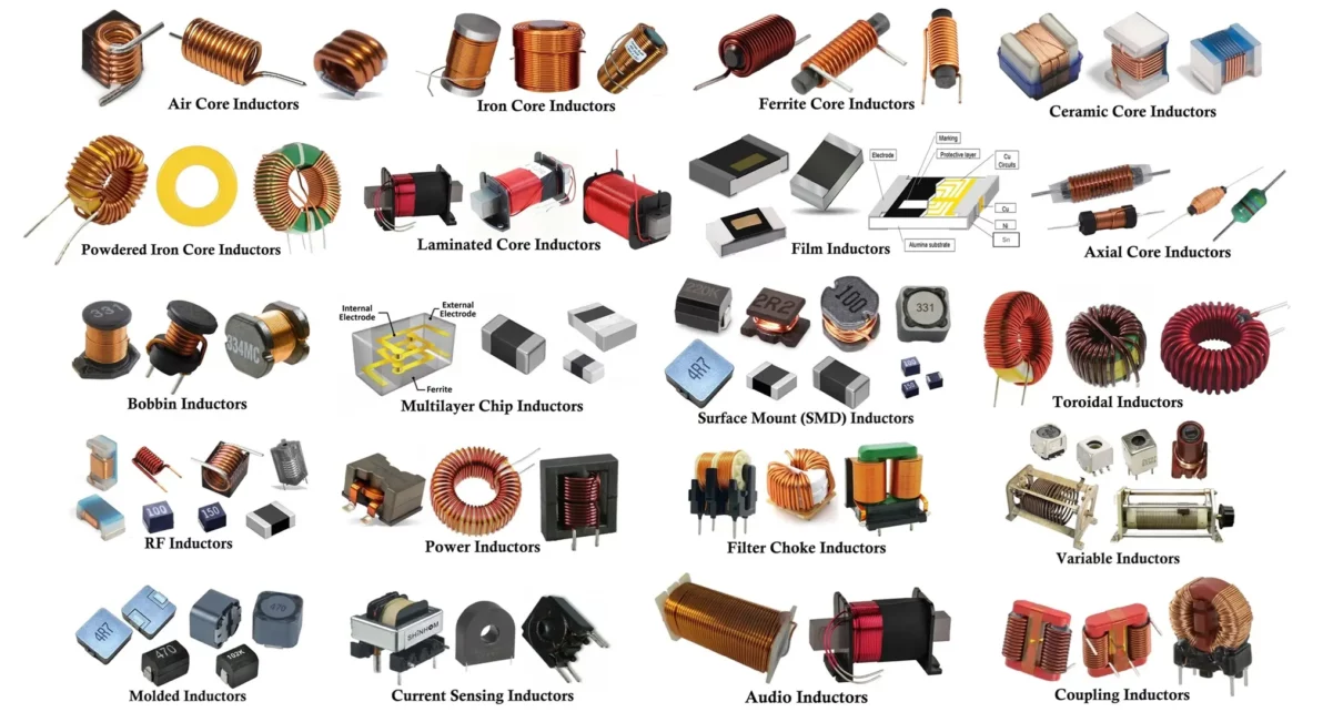
Different types of inductors. Image credit: hackatronic.com
The wires connecting the components are assumed to be ideal conductors, meaning they have negligible resistance and do not affect the circuit’s behavior. This leads us to the notion of an open circuit and a short circuit.


Figure 5:Short circuit and open circuit conditions for ideal wires.
So all points along a wire (short circuit) have the same electric potential.
Our final components are the voltage and current sources, which impose a specific voltage or current in the circuit, respectively. Here are the symbols we will use for these sources:


Figure 6:Voltage and current source symbols.
The ideal voltage source maintains a fixed voltage between its terminals, regardless of the current flowing through it. The ideal current source maintains a fixed current through it, regardless of the voltage across it. Note that the “+” and “–” signs on the voltage source indicate the polarity of the voltage (), while the arrow on the current source indicates the direction of the current flow.
More about the origin of units and symbols
We use as the symbol for inductance in honor of Emil Lenz, the physicist associated with Lenz’s law.
We don’t use for inductance because is already used to denote current. Why not use for current? Because is already used for capacitance!
Many electrical engineering conventions have roots in French terminology, reflecting the influence of French scientists and engineers in early electromagnetism. The choice of for current comes from the French word intensité (as in intensité du courant), meaning “current intensity.” The choice of or for electric charge comes from the French word quantité (as in quantité de fluide électrique), meaning “quantity of electrical fluid.” The “electricity as a fluid” analogy was strong even in the beginning!
Most symbols for electrical quantities have historical origins, often tied to the scientists who first studied or formalized these concepts.
The coulomb (C), the unit of electric charge, is named after Charles-Augustin de Coulomb, the French physicist who formulated Coulomb’s law describing the electrostatic force between charged particles.
The ampere (A), the unit of electric current, is named after André-Marie Ampère, the French physicist and mathematician who is considered one of the founders of electromagnetism.
The volt (V), the unit of electric potential, is named after Alessandro Volta, the Italian physicist who invented the first chemical battery.
The ohm (Ω), the unit of electrical resistance, is named after Georg Simon Ohm, the German physicist who formulated Ohm’s law.
The farad (F), the unit of capacitance, is named after Michael Faraday, the English scientist who made significant contributions to electromagnetism and electrochemistry.
The henry (H), the unit of inductance, is named after Joseph Henry, the American scientist who discovered electromagnetic induction independently of Faraday.
Pedantic side-note: We do not capitalize unit names derived from scientists’ names (volt, ampere, newton, kelvin, watt, ohm, henry, farad, etc.), but we do capitalize their corresponding symbols (V, A, N, K, W, Ω, H, F, etc.). The only exception is temperature: we write “degrees Celsius” (°C) and “degrees Fahrenheit” (°F), where the unit is degree (lower case) and Celsius/Fahrenheit are capitalized because they are proper names. This used to be the case for “degrees Kelvin” as well, but it was changed at the 13th General Conference on Weights and Measures in 1967 to match the naming convention used for other SI units. It is now incorrect to say “200 degrees Kelvin” or to write “200 °K.” The correct phrase is “200 kelvins” (200 K), the same way you would say “200 volts.”
Analysis of RLC circuits
Analyzing a circuit involves finding differential equations that describe the dynamics of the circuit. The quantities of interest are typically the voltages at various nodes in the circuit or the currents through various components. As with mechanical systems, we will write and rather than and to keep the notation uncluttered.
First, a bit of terminology:
A node is a point where two or more circuit elements connect. If strictly more than two elements connect at a node, we call it a junction.
A branch is a single circuit element (resistor, capacitor, inductor, voltage source, current source) connecting two nodes.
A mesh (or loop) is any closed path in the circuit.
If you are familiar with graph theory, a circuit can be represented as a graph where nodes are vertices, branches are edges and meshes are cycles.
The main variables we care about in a circuit are:
Node voltages. The electric potential at each node in the circuit.
Branch currents. The current flowing through each branch (circuit element).
To analyze a circuit, we need to set up a system of equations that relate these variables to each other. We will describe one way to do this, but there are many others!
We will illustrate our methodology with an example circuit in the next section.
Example: series RLC circuit
Consider the following series RLC circuit with a voltage source shown in the figure below. Solve for an equation that describes the current flowing through the circuit when a voltage is applied.


Figure 7:Simple RLC circuit with a voltage source. We labeled nodes , , , and branch current .
We started by labeling the nodes , , , . We chose to be ground since it is at the base of the voltage source, but we could have picked any other node. Since the same current flows through all components in this series circuit, we only need to label one branch current, which we called , and indicated it with a clockwise arrow showing the direction.
Following our methodology, we write down the constitutive equation for each component.
There are no junction nodes in this circuit, so we do not need to write any KCL equations. The first and last equation should actually be written as and , but since we set V (ground), we can simplify them as shown above.
Examining Eq. (1), we see that we have four equations and four unknowns: , , , . We do not treat the input voltage as an unknown since it is specified by the voltage source (our solution will be in terms of ).
Since we are interested in finding a single equation for the current , we can eliminate , and from the equations by summing the last three equations and eliminate by substituting in the first equation. We obtain:
We can take derivatives of both sides to obtain a second-order ordinary differential equation (ODE) for the current :
We use the traditional notation for derivatives of current because the symbol for current already has a dot on it, so we want to avoid any confusion.
Another way to write this equation is in terms of the charge that has flowed through the circuit, where . Substituting this into Eq. (2), we get:
Eqs. (3) and (4) describe the dynamics of the series RLC circuit in terms of either the current or the charge . The form of Eq. (4) is analogous to the equation of motion for a spring-mass-damper, where corresponds to mass, to damping, and to stiffness.
Example: circuit with two loops
Here is a slightly more complex example with two loops. This time, we cannot assume that the current is the same through all components, so we label each branch current separately. Our goal this time is to find an equation that describes the node voltage when a current is applied at the current source.


Figure 8:Circuit with two loops. We labeled nodes , and branch currents , , .
This time, we could not use a single loop since some of the current flows through the inductor branch while some flows through the branch. Therefore, we labeled each branch current separately. We also labeled nodes and . The node at the bottom is ground, so no need to label it. Proceeding as before, we write the constitutive equations for each component. This time, we also have a junction (node ) where three branches meet, so we will need to write a KCL equation as well.
We have five equations and five unknowns: , , , , . Since our goal is to have a single equation in terms of , we will need to eliminate all the currents. The easiest way to do this is to solve for each current in the first, third, and fourth equation and substitute into the KCL equation. This produces:
We can differentiate both sides to obtain a first-order ODE for :
Note that we didn’t use the second equation in (5) since it was not needed to eliminate the currents and obtain an equation for . However, if we wanted to find as well, we would need to use the second equation.
Test your knowledge
Solution to Exercise 1 #
Let’s start by labeling our diagram with node voltages and branch currents. The only node that needs to be labeled is the bottom one, since the top one will just be . We will call the bottom node . We will also label the branch currents as shown below.


Figure 10:RLC circuit from Figure 9 with labeled nodes and branch currents.
Now we can write the constitutive equations for each component, along with the KCL equation at node and the definition of .
We have five equations in five variables: , , , , and . Our goal is to eliminate all variables except for so we obtain a single ODE relating to .
Let’s start by eliminating by rewriting the last equation as and substituting it into the first three equations:
Solve for the current in the first three equations and substitute into the last equation:
Now differentiate to get rid of the integral and rearrange to obtain the final answer: