Bode plots - System Analysis and Control

In the previous section, we introduced the concept of frequency response. For a system with transfer function $G(s)$ , the frequency response is given by $G(j\omega)$ and tells us how the system responds to sinusoidal inputs of frequency $\omega$ . The frequency response is most useful when written in polar form as

G(j\omega) = M(\omega)\,e^{j\phi(\omega)} \quad \begin{cases} M(\omega) = |G(j\omega)| & \textsf{magnitude} \\ \phi(\omega) = \angle G(j\omega) & \textsf{phase} \end{cases}

(1)

If the input is $u(t) = \sin(\omega t)$ , then the steady-state output is a sinusoid of the same frequency, given by $y(t) = M(\omega)\sin(\omega t + \phi(\omega))$ . In other words, the system scales the input by $M(\omega)$ and shifts it in time by $\phi(\omega)$ .

Bode plots¶

It is useful to plot the frequency response as a function of $\omega$ , as this allows us to evaluate the behavior of a system at a glance. There is a standardized way of plotting the frequency response, which is called a Bode plot.

The Bode plot consists of two separate plots stacked vertically. Here is the Bode plot for the system $G(s) = \frac{1}{s+1}$ , which we will use as a running example.

Bode plot for the system G(s) = \frac{1}{s+1}. The top plot is the magnitude plot and the bottom plot is the phase plot. — Figure 1:Bode plot for the system $G(s) = \frac{1}{s+1}$ . The top plot is the magnitude plot and the bottom plot is the phase plot.

Let’s unpack Figure 1 a bit.

The top plot is the magnitude plot; it is a plot of $M(\omega)$ .
The bottom plot is the phase plot; itis a plot of $\phi(\omega)$ .
The x-axis is $\omega$ (frequency, typically in rad/s) and it is plotted on a logarithmic scale (more on this later!). The magnitude and phase plots use a common frequency axis so that it is easy to read off the magnitude and phase at a given frequency.
Each factor of 10 on the frequency axis is called a decade. This plot spans four decades, from 0.01 rad/s to 100 rad/s.
The magnitude is plotted in decibels (dB), which is a logarithmic unit. We will devote a section to explaining decibels so don’t worry!
The phase is plotted in degrees on a linear scale. Negative values correspond to phase lag while positive values correspond to phase lead.

Review of logarithmic scales¶

Logarithmic scales are useful for plotting quantities that are (1) positive and (2) vary over several orders of magnitude, which is often the case for frequency responses.

On a linear scale, the distance between any two numbers is proportional to their difference. For example, the distance between 1 and 2 is the same as the distance between 30 and 31. Here is an example of a linear scale:

Linear scales can also capture negative numbers, but they struggle to capture large ranges. For example, if we wanted to plot 0.01, 0.1, and 100, we would have to choose a scale that is large enough to include 100, which would make the points for 0.01 and 0.1 very close together and hard to read.

On a logarithmic scale, the distance between any two numbers is proportional to their ratio. For example, the distance between 1 and 3 is the same as the distance between 10 and 30, since both pairs have a ratio of 3. Here is an example of a logarithmic scale:

For example, 1,2,4,8 are equally spaced (factors of 2), and so are 1,3,9 (factors of 3). Similarly, the distance between 1 and 5 is the same as the distance between 2 and 10, since both pairs have a ratio of 5. Log scales cannot capture negative numbers, but they can capture large ranges of positive numbers. Here is the above scale extended in both directions:

Major ticks are drawn at powers of 10 (which are called decades), while minor ticks are drawn at intermediate values. For example, the ticks between 10^-1 and 10⁰ correspond to {0.2, 0.3, 0.4, 0.5, 0.6, 0.7, 0.8, 0.9}, while the minor ticks between 10¹ and 10² correspond to {20, 30, 40, 50, 60, 70, 80, 90}.

Intermediate values on a log scale¶

On a linear scale, the midpoint between $a$ and $b$ is simply $\frac{a+b}{2}$ . This is known as the arithmetic mean.

On a log scale, we have to be a bit more careful. If $x$ is the midpoint between $a$ and $b$ on a log scale, then the ratio of $a$ to $x$ must be the same as the ratio of $x$ to $b$ . Therefore,

\frac{a}{x} = \frac{x}{b} \implies x^2 = ab \implies x = \sqrt{ab}

(2)

So on a log scale, the midpoint between $a$ and $b$ is $\sqrt{ab}$ , which is the geometric mean of $a$ and $b$ . For example, the midpoint between 1 and 10 is $\sqrt{10} \approx 3.16$ .

Likewise, we can show that if $x$ is a fraction $\alpha$ of the way from $a$ to $b$ , then:

On a linear scale, $x = (1-\alpha)a + \alpha b$ .
On a log scale, $x = a^{1-\alpha}\cdot b^\alpha$ .

Logarithmic scales and music¶

What makes musical notes sound different is their pitch (frequency). Logarithmic scales are important in music, because the human ear perceives changes in pitch on a logarithmic scale.

There are many conventions associated with musical notes, but once you get past the jargon, it’s really just a logarithmic scale of frequencies! For more details, expand the section below.

Logarithmic scales and music

One octave represents a doubling or halving of frequency. This is analogous to how a decade represents a tenfold increase or decrease in frequency.

Each octave is divided into 12 semitones, which are equally spaced (called a “half-step”) on a logarithmic scale. The semitones are named C, C♯/D♭, D, D♯/E♭, E, F, F♯/G♭, G, G♯/A♭, A, A♯/B♭, B. The note “C♯/D♭” is called “C sharp” (one half-step above C) or “D flat” (one half-step below D). Two half-steps is a “whole step”, which means C and D are a whole step apart, while E and F are only a half-step apart. On a piano, the white keys correspond to the “natural” notes (C, D, E, F, G, A, B) and the black keys correspond to the sharp/flat notes (C♯/D♭, D♯/E♭, F♯/G♭, G♯/A♭, A♯/B♭). The pattern of white and black keys repeats every octave. Here is what it looks like on a piano layout.

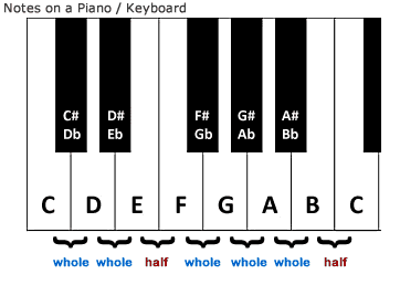
Piano keyboard — Figure 5:Partial piano keyboard layout showing the pattern of white and black keys. The pattern repeats every octave. Source: Bell&Co Music.

The octaves are numbered, so if we start at C4 (also called “middle C”), the next semitone is C♯4/D♭4, then D4, and so on until we reach B4. The next semitone after B4 is C5, which starts the next octave. A standard piano has 88 keys, starting at A0 and ending at C8.

So what are the frequencies of the musical notes? The note A4 is commonly used as a reference pitch and is set to 440 Hz. Therefore, A3 (one octave below A4) is 220 Hz, and A5 (one octave above A4) is 880 Hz. Since there are 12 semitones in an octave, the frequency of each semitone is given by multiplying the previous semitone by $2^{1/12} \approx 1.0595$ . For example, middle C (C4) is 9 semitones below A4, so its frequency is given by

f_\text{C4} = 2^{-9/12} \cdot 440 \text{ Hz} \approx 261.63 \text{ Hz}

(3)

The range of human hearing is typically considered to be from 20 Hz to 20 kHz, which corresponds to about 10 octaves. The lowest note on a standard piano (A0) is 27.5 Hz, and the highest note (C8) is 4186 Hz, which is well within the range of human hearing.

Decibels and common values¶

The magnitude in a Bode plot is typically plotted in decibels (dB), which is a logarithmic unit. The decibel value of a magnitude $M$ is given by

M_\text{dB} = 20\log_{10}(M)

(4)

Since decibels are so ubiquitous, it is useful to memorize some common values. The following table gives some common values of $M$ and their corresponding decibel values:

Common magnitudes and their corresponding decibel values

$\M$	$\M_\text{dB}$
$0$	$-\infty \text{ dB}$
$0.001$	$-60 \text{ dB}$
$0.01$	$-40 \text{ dB}$
$0.1$	$-20 \text{ dB}$
$0.5$	$\approx -6 \text{ dB}$
$1/\sqrt{2} \approx 0.707$	$\approx -3 \text{ dB}$
$1$	$0 \text{ dB}$
$\sqrt{2} \approx 1.414$	$\approx 3 \text{ dB}$
$2$	$\approx 6 \text{ dB}$
$10$	$20 \text{ dB}$
$100$	$40 \text{ dB}$
$1000$	$60 \text{ dB}$
$\infty$	$\infty \text{ dB}$

In other words, every time the magnitude is multiplied by 10, the decibel value increases by 20 dB. Likewise, every time the magnitude is doubled, the decibel value increases by approximately 6 dB.

Why are decibels defined this way?

One decibel is defined as one tenth of a bel, which is a unit named after Alexander Graham Bell, inventor of the telephone. Bell was interested in measuring how signals attenuate as they travel through telephone lines, and this was conveniently expressed as the ratio of the output power to the input power. To cover a wide range of power ratios, Bell used a logarithmic scale, which we now call the “bel”:

\text{ bel} = \log_{10}\left(\frac{P_\text{out}}{P_\text{in}}\right) = \log_{10}\left(\frac{V_\text{out}^2}{V_\text{in}^2}\right) = 2\log_{10}\left(\frac{V_\text{out}}{V_\text{in}}\right).

(5)

This is because power is proportional to the square of the voltage (or current). If we then want to convert to decibels, we multiply by 10. So if voltage is amplified by a factor of $M$ , this amplification in decibels (dB) is given by:

\boxed{M_\text{dB} = 20\log_{10}(M)}

(6)

Decibels and sound intensity¶

The decibel scale is also used to measure the loudness of sound. The reference value is typically the threshold of human hearing, which is around 20 μPa^[1]. For example, a whisper is around 30 dB, normal conversation is around 60 dB, and a rock concert can be around 120 dB. The decibel scale allows us to express a wide range of sound intensities in a compact way. This means that the pressure wave of a rock concert is 1,000 times stronger than that of a normal conversation.

Interpreting a Bode plot¶

Let’s return to the bode plot for the system $G(s) = \frac{1}{s+1}$ and see how to read it.

The Bode plot of Figure 6 spans 4 decades (10^-2 to 10² rad/s). We can read off some key features of the system from the plot:

DC gain: The DC gain is $G(0)$ , which is the frequency response at $\omega=0$ . Although the Bode plot does not show $\omega=0$ (that would be infinitely far to the left due to the log scale), we can see that as $\omega\to 0$ , we have $M \to 0\text{ dB}$ and $\phi \to 0\degree$ . So the DC gain is 0 dB, which corresponds to a magnitude of 1. We can verify this from the transfer function: $G(0) = \frac{1}{0+1} = 1$ . Magnitude is always positive, so if the system had been $\frac{-1}{s-1}$ (DC gain of -1), the magnitude plot would look the same, but the phase plot would show a phase of -180° instead of 0° at low frequencies, which would tell us that the sign of the DC gain should be flipped.
High-frequency roll-off: All Bode magnitude plots for physical systems eventually have a constant-slope magnitude plot at high frequency, which is called the high-frequency roll-off. For the plot above, the high-frequency roll-off is -20 dB/decade.
Corner frequency: When the Bode plot has a frequency where the magnitude transitions from flat to sloped, this frequency is called the corner frequency (also called the break frequency or cutoff frequency). The plot above has a corner frequency at 1 rad/s. This means that the system behaves like a low-pass filter, allowing low frequencies to pass through while attenuating frequencies that are larger than the corner frequency.

We can also read off specific values from the plot and deduce what this means in terms of steady-state response. For example:

At $\omega = 0.01 \text{ rad/s}$ , the magnitude is approximately 0 dB, or 1, and the phase is approximately 0°. This means that the output is essentially unchanged.

\begin{aligned} u(t) &= \cos(0.01 t) \\\implies\; y(t) &\approx 1\cdot \cos(0.01 t + 0\degree) = \cos(0.01 t) \end{aligned}

(7)

At $\omega = 1 \text{ rad/s}$ , the magnitude is approximately -3 dB, or 0.707, and the phase is approximately -45°. This means that the output is attenuated by a factor of 0.707 and lags the input by 45°. For example:

\begin{aligned} u(t) &= \cos(t) \\\implies\; y(t) &\approx 0.707\cdot \cos(t - 45\degree) \end{aligned}

(8)

At $\omega = 100 \text{ rad/s}$ , the magnitude is approximately -40 dB, or 0.01, and the phase is approximately -90°. This means that the output is attenuated by a factor of 0.01 and lags the input by 90°. For example:

\begin{aligned} u(t) &= \cos(100 t) \\\implies\; y(t) &\approx 0.01\cdot \cos(100 t - 90\degree) = 0.01\cdot \sin(100 t) \end{aligned}

(9)

Experimentally measuring a Bode plot¶

In practice, we often do not have access to the transfer function of a system, but we can still measure its frequency response and plot its Bode plot. To do this, we can apply sinusoidal inputs of different frequencies to the system and measure the steady-state output. For each input frequency $\omega$ , we can compute the magnitude $M(\omega)$ and phase $\phi(\omega)$ from the input and output signals, plot them, and connect the dots.

This approach only works if the system is stable, since otherwise the output will not settle to a steady-state sinusoid.

Test your knowledge¶

Solution to Exercise 1 #

The DC gain is the magnitude at $\omega \to 0$ . From the plot, we can see that as $\omega \to 0$ , the magnitude approaches -20 dB, which corresponds to a magnitude of 0.1. Therefore, the DC gain is 0.1.
The high-frequency roll-off is the slope of the magnitude plot at high frequencies. From the plot, we can see that the magnitude decreases from -40 dB to -80 dB during the final decade, which corresponds to a roll-off of -40 dB/decade.
The corner frequency, where the initial flat portion and the high-frequency roll-off intersect, is roughly at $\omega = 3$ rad/s.

To observe the maximum amplification in the response, we should use a sinusoidal input at the resonance frequency, which is approximately equal to the corner frequency of 3 rad/s. At this frequency, we have $M \approx -14 \text{ dB}$ . Since this is about 6 dB (factor of 2) larger than -20 dB (factor of 0.1), we have a net gain of 0.2. We also have $\phi \approx -90\degree$ . Two possible examples are:

Using $u(t) = \sin(3 t)$ would yield $y(t) \approx 0.2 \sin(3 t - 90\degree)$ .
Using $u(t) = \cos(3 t)$ would yield $y(t) \approx 0.2 \cos(3 t - 90\degree)$ .

Solution to Exercise 2 #

We want the largest note that is less than or equal to 20 kHz. The frequency of the $n^\text{th}$ semitone above A4 is given by

f_n = 440 \cdot 2^{n/12}

(10)

We want to find the largest $n$ such that $f_n \leq 20{,}000$ Hz. Solving for $n$ , we get

\begin{aligned} n &\leq 12 \log_2\left(\frac{20{,}000}{440}\right) \\ &\approx 12 \log_2(45.45) \\ &\approx 12 \cdot 5.51 \\ &\approx 66.1 \end{aligned}

(11)

The largest integer $n$ that satisfies this is $n=66$ . Each octave has 12 semitones, so 66 semitones equals 5 octaves plus 6 semitones. We started at A4, so adding 5 octaves brings us to A9. Writing out the next six semitones (using Figure 5 as a reference), we get the following notes:

A9, A♯9/B♭9, B9, C10, C♯10/D♭10, D10, D♯10/E♭10, ...

Therefore, the highest note that a human can hear is D♯10/E♭10, which has a frequency of approximately $440 \cdot 2^{66/12} \approx 19{,}912$ Hz.

Footnotes¶

MicroPascals, measuring the root-mean-square pressure amplitude of a 1 kHz sound wave at the threshold of human hearing.
↩