Linearization

Smooth functions look like straight lines when you zoom in close enough to any point. It turns out something similar is true of dynamical systems. If we “zoom in close enough,” it will look like a linear system. In this section, we will make this idea precise and show how to derive linear approximations of nonlinear dynamical systems.

Linearizing a function¶

Linearization is an approximation method. Given a function $f(x)$, consider a reference point $x_0$. If $f$ is a smooth function, $f(x)$ near $x=x_0$ drawing a tangent line on the graph and using the line as the approximation. The line will have slope $f'(x_0)$, so the linear approximation will have equation:

We can write this another way. Define $y=f(x)$ and $y_0=f(x_0)$. Then define the deviations from the reference point as

and we can write our linearized equation as:

Now it truly looks like a linear equation $y=kx$, but it is linear in the deviations from the reference point. It is not linear in the original coordinates $(x,y)$.

Example: approximating the square root¶

Let’s approximate $\sqrt{4.01}$ via linearization.

We know that $4.01$ is close to $4$ and $\sqrt{4}=2$, so let’s set $f(x) = \sqrt{x}$ and pick the reference point $x_0=4$. Then we have $f(x_0) = \sqrt{4} = 2$ and $f'(x) = \frac{1}{2\sqrt{x}}$, so $f'(x_0) = \frac{1}{2\cdot 2} = \frac{1}{4}$. Therefore, our linearized approximation near $x_0=4$ is:

In our example, $\delta x = 0.01$, so we have $\sqrt{4.01} \approx 2.0025$.

The true value is $\sqrt{4.01} \approx 2.002498$, so our approximation is quite accurate!

Multivariable functions¶

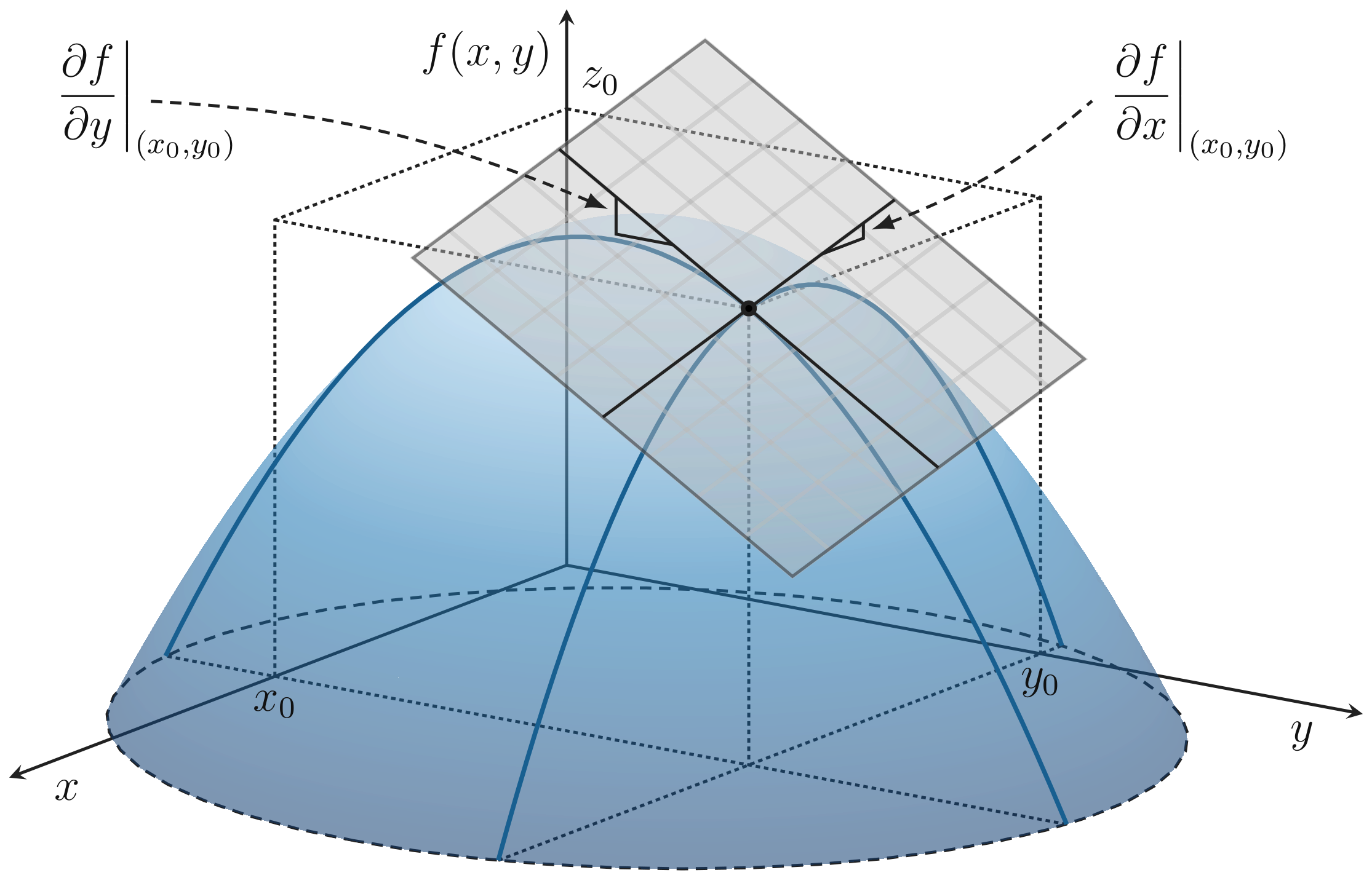
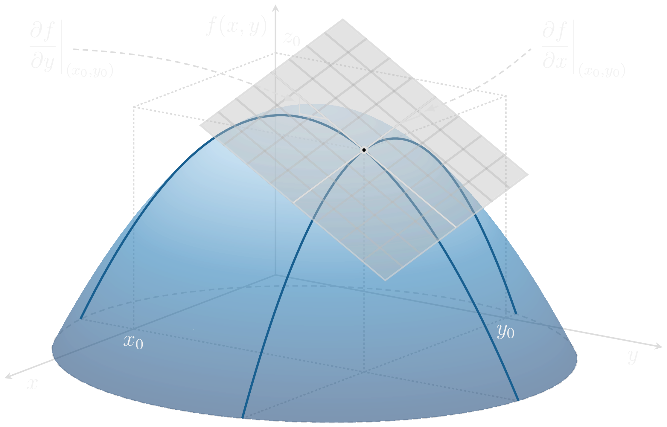
We can make an analogous approximation for multivariable functions, except we approximate the function using a tangent hyperplane rather than a tangent line. For example, for a function $f(x,y)$, we can approximate it about the point $(x_0,y_0)$ as

where we use the notation $\left.\frac{\partial f}{\partial x}\right|_0$ to mean “take the partial derivative of $f(x,y)$ with respect to $x$ and then evaluate the result at $x=x_0$ and $y=y_0$”. Setting $z=f(x,y)$ and $z_0=f(x_0,y_0)$ and defining the deviations $\delta x$, $\delta y$, $\delta z$ analogously as before, our linearized equation becomes

Equilibrium points¶

For example, consider the pendulum of Eq. (3).

An equilibrium point $(\theta_0,T_0)$ is a constant angle $\theta_0$ and constant torque $T_0$ that satisfies (7). All time derivatives vanish and we are left with the equation of motion, we have

There are many ways to satisfy Eq. (8). Each is a valid equilibrim point.

• Pick $\theta_0=0$ and $T_0=0$. The pendulum is pointing down and we apply no torque.

• Pick $\theta_0=\pi$ and $T_0=0$. The pendulum is pointing up and we apply no torque.

• Pick $\theta_0=\tfrac{\pi}{4}$ and $T_0=\tfrac{1}{\sqrt{2}}mg\ell$. The pendulum is perfectly balanced at 45°.

• Pick any $\theta_0$ and use $T_0=mg\ell\sin\theta_0$.

In all cases, if we use $\theta(0)=\theta_0$ as an initialization and apply the equilibrium torque $T(t)=T_0$ for all $t\geq 0$, the pendulum will remain at the angle $\theta(t)=\theta_0$ for all $t\geq 0$.

We typically find equilibrium points in one of two ways. If the system in question has input $u$ and other signals $x$, then:

1. We are interested in the zero-input equilibrium, so we use $u_0=0$ and we ask what values of $x_0$ are possible. This is what we did for the first two equilibrium examples for the pendulum above.

2. We pick a desired $x_0$, and we ask what is the required $u_0$ that will lead to equilibrium. This is what we did for the last two equilibrium examples for the pendulum above.

Linearizing a dynamical system¶

To linearize a non-LTI system, we carry out the following steps. We will assume the system has inputs $\u = [u_1,\dots,u_m]$ and other signals $\x = [x_1,\dots,x_n]$ (we use the boldface letters to denote vectors).

We will spend the rest of this section doing specific examples to understand how to derive linearized approximations in practice.

Example: gravity shift¶

Consider a spring-mass system under the effect of a force $F$ and also gravity.

If we imagine that the spring is at rest without gravity then the equations of motion are:

This equation is not linear due to the affine term $mg$. So let’s linearize!

We want the system to be at rest when $F=0$ (no applied force), so let’s pick $F_0=0$ and see what $x_0$ must be. Substituting into the equation of motion, we have

Therefore $x_0=\frac{mg}{k}$. This is where the mass will sit so that the spring force perfectly balances out the force of gravity.

Our equation of motion (11) is already affine, so we don’t need to take any derivatives. We can simply substitute our deviations from equilibrium: $x = x_0 + \delta x$ and $F = F_0 + \delta F = \delta F$. Substituting into (11), we have

The constant terms cancel out $(kx_0 = mg)$ because of how we chose $x_0$ in (12) and we are left with

This is an LTI system in the variables $(\delta x, \delta F)$. In fact, it looks very similar to our original equations of motion (11), except that the gravity term is gone.

What happened physically? We shifted our coordinate system down by $\frac{mg}{k}$, so that the new “zero” position is where the mass naturally sits under gravity. In this new coordinate system, there is no gravity term, and if we apply a force from this new “zero” position, the mass will move up or down the same way as without gravity, except shifted down by $\frac{mg}{k}$. The equations of motion (14) describe exactly this behavior.

Example: cruise control¶

Consider a car moving along a flat road. The motor provides a forward force $F_a$ and the aerodynamic drag provides an opposing force $F_d$. Let’s derive linearized equations of motion linearized about a nominal speed $v_0$.

Aerodynamic drag is typically proportional to the square of the speed of the object. This drag force is given by the equation

where $C_d$ is the drag coefficient, $\rho$ is the air density, $A$ is the lateral surface area, and $v$ is the speed of the moving object. We replaced all the constant terms by $c$ for simplicity. The equation of motion for the car is therefore

This is not linear due to the $v^2$ term. Let’s linearize about the nominal speed $v_0$. We will carefully follow the four steps outlined earlier.

Step 1: Let’s identify an equilibrium point. In order to maintain a constant speed $v_0$, what must be the applied force $F_a$? We can substitute into the equation of motion to obtain:

Step 2: Now we linearize all nonlinear terms. The only nonlinear term is the drag force $cv^2$. Linearize this about $v_0$ using Eq. (1):

Substituting this into our equation of motion, we obtain

Step 3: Now we replace all signals with their deviations from equilibrium: $v = v_0 + \delta v$ and $F_a = F_0 + \delta F$. Also use the fact that $\dot v = \delta \dot v$ because $v_0$ is constant. Substituting, we have

Step 4: Finally, we can cancel out the nominal force terms using (17) and we obtain our linearized equation of motion.

We can quickly check that this is indeed LTI: all terms are linear functions of the deviations $\delta v$ and $\delta F$.

We can also interpret this result physically. Our linearized equation (21) relates the deviation from $F_0$ to the deviation from $v_0$. If we let $\delta v = \delta \dot x$, we can write it as an equation in terms of position:

This is a spring-mass-damper equation with no spring! Moreover, the damping coefficient depends linearly on the nominal velocity: the faster you go, the more damping you have. Makes sense!

Example: pendulum¶

Returning to the pendulum example illustrated below, let’s find the linearized equations of motion about an arbitrary equilibrium angle $\theta_0$.

As mentioned earlier, the equation of motion is

Step 1: First, we find the equilibrium torque. As computed earlier,

Step 2: Next, we linearize the nonlinear term about $\theta_0$:

Substituting into the equation of motion (23), we obtain

Step 3: Now substitute $T = T_0 + \delta T$ and $\theta = \theta_0 + \delta\theta$ and obtain

Step 4: We can apply (24) to cancel the nominal torque and we get

This is an LTI system in the variables $(\delta \theta, \delta T)$, so our linearization is complete!

We can investigate what happens when we use different equilibrium points:

• If $\theta_0=0$ (pendulum pointing down), we get $m\ell^2\delta\ddot \theta + mg\ell \delta\theta = \delta T$. This is just what you get when you apply the “small angle formula” $\sin\theta \approx \theta$. Indeed, the small angle formula is simply linearization about zero. The linearized equation of motion is the same as that of a standard spring-mass system.

• If $\theta_0=\pi$ (pendulum pointing up), we get $m\ell^2\delta\ddot \theta - mg\ell \delta\theta = \delta T$. This looks similar to the standard linearized pendulum, but with an important negative sign. This is like a spring-mass system with a negative spring constant. When you push the mass, it accelerates away from you rather than returning back.

• If $\theta_0=\tfrac{\pi}{4}$ (pendulum at 45 degrees), we get $m\ell^2\delta\ddot \theta + \tfrac{1}{\sqrt{2}}mg\ell \delta\theta = \delta T$. It’s a spring-mass system with a reduced spring constant.

Test your knowledge¶